Softmax Regression
转自: http://ufldl.stanford.edu/wiki/index.php/Softmax_Regression
Softmax Regression
Softmax Regression
Contents[hide] |
Introduction
In these notes, we describe the Softmax regression model. This model generalizes logistic regression to classification problems where the class label y can take on more than two possible values. This will be useful for such problems as MNIST digit classification, where the goal is to distinguish between 10 different numerical digits. Softmax regression is a supervised learning algorithm, but we will later be using it in conjuction with our deep learning/unsupervised feature learning methods.Recall that in logistic regression, we had a training set
 of m labeled examples, where the input features are
  .
(In this set of notes, we will use the notational convention of letting the feature vectors x be
n + 1 dimensional, with x0 = 1 corresponding to the intercept term.)
With logistic regression, we were in the binary classification setting, so the labels
were
.
(In this set of notes, we will use the notational convention of letting the feature vectors x be
n + 1 dimensional, with x0 = 1 corresponding to the intercept term.)
With logistic regression, we were in the binary classification setting, so the labels
were  . Our hypothesis took the form:
and the model parameters θ were trained to minimize the cost function
![\begin{align}
J(\theta) = -\frac{1}{m} \left[ \sum_{i=1}^m y^{(i)} \log h_\theta(x^{(i)}) + (1-y^{(i)}) \log (1-h_\theta(x^{(i)})) \right]
\end{align}](http://ufldl.stanford.edu/wiki/images/math/f/a/6/fa6565f1e7b91831e306ec404ccc1156.png)
In the softmax regression setting, we are interested in multi-class classification (as opposed to only binary classification), and so the label y can take on k different values, rather than only two. Thus, in our training set
,
we now have that  . (Note that
our convention will be to index the classes starting from 1, rather than from 0.) For example,
in the MNIST digit recognition task, we would have k = 10 different classes.
. (Note that
our convention will be to index the classes starting from 1, rather than from 0.) For example,
in the MNIST digit recognition task, we would have k = 10 different classes.
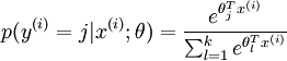
Given a test input x, we want our hypothesis to estimate the probability that p(y = j | x) for each value of
 .
I.e., we want to estimate the probability of the class label taking
on each of the k different possible values. Thus, our hypothesis
will output a k dimensional vector (whose elements sum to 1) giving
us our k estimated probabilities. Concretely, our hypothesis
hθ(x) takes the form:
.
I.e., we want to estimate the probability of the class label taking
on each of the k different possible values. Thus, our hypothesis
will output a k dimensional vector (whose elements sum to 1) giving
us our k estimated probabilities. Concretely, our hypothesis
hθ(x) takes the form:
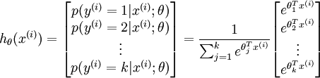
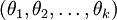
Here
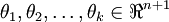 are the
parameters of our model.
Notice that
the term
are the
parameters of our model.
Notice that
the term  normalizes the distribution, so that it sums to one.
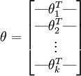
For convenience, we will also write θ to denote all the parameters of our model. When you implement softmax regression, it is usually convenient to represent θ as a k-by-(n + 1) matrix obtained by stacking up
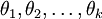 in rows, so that
Cost Function
We now describe the cost function that we'll use for softmax regression. In the equation below, is
the indicator function, so that 1{a true statement} = 1, and 1{a false statement} = 0.
For example, 1{2 + 2 = 4} evaluates to 1; whereas 1{1 + 1 = 5} evaluates to 0. Our cost function will be:
is
the indicator function, so that 1{a true statement} = 1, and 1{a false statement} = 0.
For example, 1{2 + 2 = 4} evaluates to 1; whereas 1{1 + 1 = 5} evaluates to 0. Our cost function will be:
![\begin{align}
J(\theta) = - \frac{1}{m} \left[ \sum_{i=1}^{m} \sum_{j=1}^{k} 1\left\{y^{(i)} = j\right\} \log \frac{e^{\theta_j^T x^{(i)}}}{\sum_{l=1}^k e^{ \theta_l^T x^{(i)} }}\right]
\end{align}](http://ufldl.stanford.edu/wiki/images/math/7/6/3/7634eb3b08dc003aa4591a95824d4fbd.png)
Notice that this generalizes the logistic regression cost function, which could also have been written:
![\begin{align}
J(\theta) &= -\frac{1}{m} \left[ \sum_{i=1}^m (1-y^{(i)}) \log (1-h_\theta(x^{(i)})) + y^{(i)} \log h_\theta(x^{(i)}) \right] \\
&= - \frac{1}{m} \left[ \sum_{i=1}^{m} \sum_{j=0}^{1} 1\left\{y^{(i)} = j\right\} \log p(y^{(i)} = j | x^{(i)} ; \theta) \right]
\end{align}](http://ufldl.stanford.edu/wiki/images/math/5/4/9/5491271f19161f8ea6a6b2a82c83fc3a.png)
The softmax cost function is similar, except that we now sum over the k different possible values of the class label. Note also that in softmax regression, we have that
 .
.
There is no known closed-form way to solve for the minimum of J(θ), and thus as usual we'll resort to an iterative optimization algorithm such as gradient descent or L-BFGS. Taking derivatives, one can show that the gradient is:
![\begin{align}
\nabla_{\theta_j} J(\theta) = - \frac{1}{m} \sum_{i=1}^{m}{ \left[ x^{(i)} \left( 1\{ y^{(i)} = j\} - p(y^{(i)} = j | x^{(i)}; \theta) \right) \right] }
\end{align}](http://ufldl.stanford.edu/wiki/images/math/5/9/e/59ef406cef112eb75e54808b560587c9.png)
Recall the meaning of the "
 " notation. In particular,
  is itself a vector, so that its l-th element is
  the partial derivative of J(θ) with respect to the l-th element of θj.
Armed with this formula for the derivative, one can then plug it into an algorithm such as gradient descent, and have it minimize J(θ). For example, with the standard implementation of gradient descent, on each iteration we would perform the update
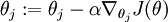 (for each ).
When implementing softmax regression, we will typically use a modified version of the cost function described above; specifically, one that incorporates weight decay. We describe the motivation and details below.
Properties of softmax regression parameterization
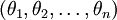
Softmax regression has an unusual property that it has a "redundant" set of parameters. To explain what this means, suppose we take each of our parameter vectors θj, and subtract some fixed vector ψ from it, so that every θj is now replaced with θj − ψ (for every). Our hypothesis
now estimates the class label probabilities as
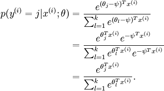
In other words, subtracting ψ from every θj does not affect our hypothesis' predictions at all! This shows that softmax regression's parameters are "redundant." More formally, we say that our softmax model is overparameterized, meaning that for any hypothesis we might fit to the data, there are multiple parameter settings that give rise to exactly the same hypothesis function hθ mapping from inputs x to the predictions.
Further, if the cost function J(θ) is minimized by some setting of the parameters
 ,
then it is also minimized by
,
then it is also minimized by  for any value of ψ. Thus, the
minimizer of J(θ) is not unique. (Interestingly,
J(θ) is still convex, and thus gradient descent will
not run into a local optima problems. But the Hessian is singular/non-invertible,
which causes a straightforward implementation of Newton's method to run into
numerical problems.)
for any value of ψ. Thus, the
minimizer of J(θ) is not unique. (Interestingly,
J(θ) is still convex, and thus gradient descent will
not run into a local optima problems. But the Hessian is singular/non-invertible,
which causes a straightforward implementation of Newton's method to run into
numerical problems.)
Notice also that by setting ψ = θ1, one can always replace θ1 with
 (the vector of all
0's), without affecting the hypothesis. Thus, one could "eliminate" the vector
of parameters θ1 (or any other θj, for
any single value of j), without harming the representational power
of our hypothesis. Indeed, rather than optimizing over the k(n + 1)
parameters (where
(the vector of all
0's), without affecting the hypothesis. Thus, one could "eliminate" the vector
of parameters θ1 (or any other θj, for
any single value of j), without harming the representational power
of our hypothesis. Indeed, rather than optimizing over the k(n + 1)
parameters (where
 ), one could instead set
  and optimize only with respect to the (k − 1)(n + 1)
remaining parameters, and this would work fine.
and optimize only with respect to the (k − 1)(n + 1)
remaining parameters, and this would work fine.
In practice, however, it is often cleaner and simpler to implement the version which keeps all the parameters
 , without
arbitrarily setting one of them to zero. But we will
make one change to the cost function: Adding weight decay. This will take care of
the numerical problems associated with softmax regression's overparameterized representation.
, without
arbitrarily setting one of them to zero. But we will
make one change to the cost function: Adding weight decay. This will take care of
the numerical problems associated with softmax regression's overparameterized representation.
Weight Decay
We will modify the cost function by adding a weight decay term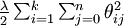 which penalizes large values of the parameters. Our cost function is now
![\begin{align}
J(\theta) = - \frac{1}{m} \left[ \sum_{i=1}^{m} \sum_{j=1}^{k} 1\left\{y^{(i)} = j\right\} \log \frac{e^{\theta_j^T x^{(i)}}}{\sum_{l=1}^k e^{ \theta_l^T x^{(i)} }} \right]
+ \frac{\lambda}{2} \sum_{i=1}^k \sum_{j=0}^n \theta_{ij}^2
\end{align}](http://ufldl.stanford.edu/wiki/images/math/4/7/1/471592d82c7f51526bb3876c6b0f868d.png)
With this weight decay term (for any λ > 0), the cost function J(θ) is now strictly convex, and is guaranteed to have a unique solution. The Hessian is now invertible, and because J(θ) is convex, algorithms such as gradient descent, L-BFGS, etc. are guaranteed to converge to the global minimum.
To apply an optimization algorithm, we also need the derivative of this new definition of J(θ). One can show that the derivative is:
![\begin{align}
\nabla_{\theta_j} J(\theta) = - \frac{1}{m} \sum_{i=1}^{m}{ \left[ x^{(i)} ( 1\{ y^{(i)} = j\} - p(y^{(i)} = j | x^{(i)}; \theta) ) \right] } + \lambda \theta_j
\end{align}](http://ufldl.stanford.edu/wiki/images/math/3/a/f/3afb4b9181a3063ddc639099bc919197.png)
By minimizing J(θ) with respect to θ, we will have a working implementation of softmax regression.
Relationship to Logistic Regression
In the special case where k = 2, one can show that softmax regression reduces to logistic regression. This shows that softmax regression is a generalization of logistic regression. Concretely, when k = 2, the softmax regression hypothesis outputs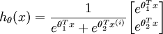
Taking advantage of the fact that this hypothesis is overparameterized and setting ψ = θ1, we can subtract θ1 from each of the two parameters, giving us
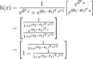
Thus, replacing θ2 − θ1 with a single parameter vector θ', we find that softmax regression predicts the probability of one of the classes as
 ,
and that of the other class as
,
and that of the other class as
 ,
same as logistic regression.
,
same as logistic regression.
Softmax Regression vs. k Binary Classifiers
Suppose you are working on a music classification application, and there are k types of music that you are trying to recognize. Should you use a softmax classifier, or should you build k separate binary classifiers using logistic regression?This will depend on whether the four classes are mutually exclusive. For example, if your four classes are classical, country, rock, and jazz, then assuming each of your training examples is labeled with exactly one of these four class labels, you should build a softmax classifier with k = 4. (If there're also some examples that are none of the above four classes, then you can set k = 5 in softmax regression, and also have a fifth, "none of the above," class.)
If however your categories are has_vocals, dance, soundtrack, pop, then the classes are not mutually exclusive; for example, there can be a piece of pop music that comes from a soundtrack and in addition has vocals. In this case, it would be more appropriate to build 4 binary logistic regression classifiers. This way, for each new musical piece, your algorithm can separately decide whether it falls into each of the four categories.
Now, consider a computer vision example, where you're trying to classify images into three different classes. (i) Suppose that your classes are indoor_scene, outdoor_urban_scene, and outdoor_wilderness_scene. Would you use sofmax regression or three logistic regression classifiers? (ii) Now suppose your classes are indoor_scene, black_and_white_image, and image_has_people. Would you use softmax regression or multiple logistic regression classifiers?
In the first case, the classes are mutually exclusive, so a softmax regression classifier would be appropriate. In the second case, it would be more appropriate to build three separate logistic regression classifiers.
Softmax Regression | Exercise:Softmax Regression
Language : 中文
- This page was last modified on 7 April 2013, at 13:24.
- This page has been accessed 224,464 times.
- Privacy policy
- About Ufldl
- Disclaimers
Labels: AI, Coding, neural networks
posted by cs @ 11:06 PM
![]()

0 Comments:
Post a Comment
Subscribe to Post Comments [Atom]
<< Home